11 M3A: Using Projects and Scripts in R
This content draws on material from:
- STAT 545 by Jenny Bryan, licensed under CC BY-SA 4.0
- Statistical Inference via Data Science: A ModernDive into R and the Tidyverse by Chester Ismay and Albert Y. Kim, licensed under CC BY-NC-SA 4.0
Changes to the source material include addition of new material; light editing; rearranging, removing, and combining original material; adding and changing links; and adding first-person language from current author.
The resulting content is licensed under CC BY-NC-SA 4.0.
11.1 Introduction
A couple of years ago, I had to make an official correction to my most-cited research study. My co-author and I were revisiting some of the calculations in the study as part of a separate project, and we found some discrepancies between the published results and the results that my co-author was getting. It turned out that back in 2017, we hadn’t been working off of the same data file when working on separate parts of the paper, and that created small-but-embarrassing inconsistencies between what we had published and what the actual results were. When you’re doing data science work, it’s very important to keep things organized!
We’ve run some code in R already, but how we manage that code can be really important. In this walkthrough, we’ll learn some more R and RStudio features before learning more about scripts and Projects in R. By way of reminder, whenever you see a “code chunk,” you should type (or copy) the code and run it on your own; however, remember also that output looks a lot like code chunks but doesn’t need to be run! Any box that immediately follows a code chunk is just output: It’s there for you to compare your results against, not for you to copy and paste. Likewise, text that is marked as code but is in the middle of a paragraph doesn’t need to be run; it’s just a way of showing that something is code.
11.2 More About R and RStudio
Begin this walkthrough by starting RStudio. By way of reminder, as you open up the program, you should see something similar to Figure 11.1.
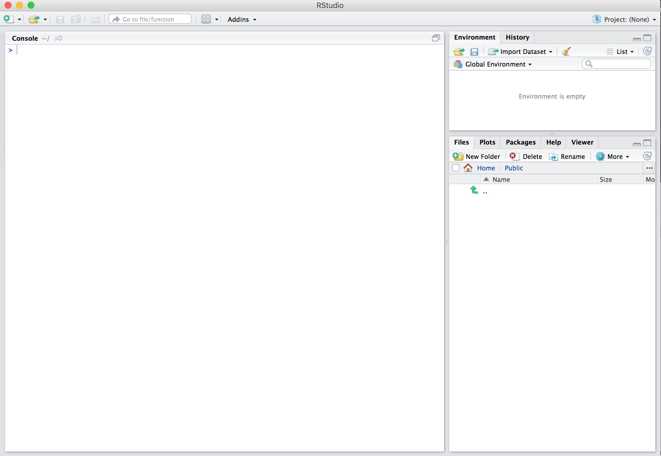
Figure 11.1: RStudio interface to R.
Note again the three panes (that is, the three panels dividing the screen):
- the console pane,
- the files pane,
- and the environment pane.
Let’s spend some more time in the Console, which is where we interact with the live R process.
The following code tells R to assign the result of 3 * 4 (that is, 3 times 4) to an object called x and then asks R to “inspect” the object (that is, retrieve its contents). Go ahead and run it on your own:
[1] 12All R statements where you create object —“assignments”—have this form: objectName <- value. It is technically possible to use = to make assignments, too, but it’s a pretty bad idea, for reasons we don’t need to go into here. Yes, it takes a bit more effort, but always make assignments with <-.
Object names cannot start with a digit and cannot contain certain other characters such as a comma or a space. It’s important to get into good habits with naming your objects. Many people use some kind of regular pattern in naming objects with multiple words: i_use_snake_case, other.people.use.periods, and evenOthersUseCamelCase
Make another assignment by running this code:
To inspect this object, try out RStudio’s completion facility: type the first few characters of this_is_a_really_long_name, press TAB, add characters until you disambiguate, then press return.
Now, make another assignment:
What happens if we try to run the following code to inspect our new object?
Error in eval(expr, envir, enclos): object 'stromaerocks' not foundThere’s an implicit contract when you work with a scripting language like R: The computer will do tedious computation for you, but you must be completely precise in your instructions. Typos matter. Case matters. Details matter. I am always happy to help you troubleshoot, but please make sure that you’ve checked the details of your code first. It’s amazing how often errors come down to mistyping something.
R has a mind-blowing collection of built-in functions that are accessed like so: functionName(argument1 = value1, argument2 = value2, and so on). The details look different from function to function, but they typically follow this pattern.
Let’s try functions using seq(), which makes regular sequences of numbers. While we’re at it, we’ll demo more helpful features of RStudio.
Type se and hit TAB. A pop up shows you possible completions. Specify seq() by typing more to disambiguate or using the up/down arrows to select. Notice the floating tool-tip-type help that pops up, reminding you of a function’s arguments. If you want even more help, press F1 as directed to get the full documentation in the help tab of the lower right pane. You can also run a function with a ? in front of it (for example, ?seq()) to bring up the same help documentation.
Now type the open parenthesis (() and notice the automatic addition of the closing parenthesis and the placement of cursor in the middle. Type the arguments 1, 10 and hit return. RStudio also exits the parenthetical expression for you. These little features are the things that can make RStudio really useful (though I’ll also admit that they sometimes get in the way, too).
[1] 1 2 3 4 5 6 7 8 9 10Note that even though we ran this function, we didn’t assign the results to an object. That means that we can see the results in the Console, but we won’t be able to retrieve them later! If we want to hold onto the results of a function, we need to assign it to an object.
Make this assignment and notice that RStudio helps with quotation marks in the same way that it helps with parentheses.
If you just make an assignment, you don’t get to see the value, so then you’re tempted to immediately inspect.
[1] 1 2 3 4 5 6 7 8 9 10This common action can be shortened by surrounding the assignment with parentheses, which causes assignment and “print to screen” to happen.
[1] 1 2 3 4 5 6 7 8 9 10Not all functions have (or require) arguments:
[1] "Mon Aug 26 16:18:39 2024"Note that the output you get after running date() ought to be different than the output above… can you figure out why?
Now look at your workspace in the upper right Environment pane. The workspace is where user-defined objects accumulate. You ought to see all of the objects that we’ve created so far in this walkthrough. You can also get a listing of these objects with these other commands:
If you want to remove the object named y, you can do this:
To remove everything:
You can also click the broom in RStudio’s Environment pane to remove everything. Sometimes this is helpful when troubleshooting code.
11.3 The Console and the Workspace
One day you will need to quit R, go do something else and return to your analysis later. One day you will have multiple analyses going that use R and you want to keep them separate. One day you will need to bring data from the outside world into R and send numerical results and figures from R back out into the world.
To handle these real life situations, you need to make two decisions:
- What from your analysis needs to be saved?
- Where does your analysis need to be saved?
In the R code that we’ve written so far, we’ve run all of our code in the Console, and it’s been saved to the workspace. This has been sufficient for how we’ve done things so far, but it’s not a great long-term solution.
Anything that we type into the Console gets saved into your “R history.” You can retrieve code from your R history by pressing the up arrow when your cursor is in the Console. This can be helpful for something you just typed, but it’s also a hassle to go all the way through your R history to find something that you typed hours (or even just minutes) ago.
When you quit RStudio, it will generally prompt you to save your workspace; if you do, it will load it back automatically for you when you next open RStudio. This is also handy, but even though you have the results of your work, you don’t have easy access to the process that you took to get there. (That is, objects in your workspace are not easily reproducible). If you need to redo analysis, you’re going to either redo a lot of typing (making mistakes all the way) or will have to mine your R history (using those arrow keys in the console) for the commands you used.
A better use of your time and psychic energy is to keep your “good” R code in a script for future reuse—and to keep your related scripts bundled together into a project. In other words, you can do one-off, temporary, or unimportant things in the Console, but most of your code is worth saving—especially if you need help troubleshooting it!
11.4 Holding Onto Code
The rest of this walkthrough will demonstrate how to write code in a way that lets you hold onto it later. This can be really helpful for you (for example, when you want to adapt code from a class activity for one of your projects), and it’s also really helpful for me (for example, when I want to see all the code you ran when helping you troubleshoot an activity).
11.4.1 RStudio Projects
Keeping all the files associated with a project organized together—input data, R scripts, analytical results, figures—is such a wise and common practice that RStudio has built-in support for this.
Let’s make a project for you to use during the rest of this semester. In RStudio, navigate to File and then New Project. When prompted, click on Existing Directory and then navigate to the folder for the GitHub repository that you created last week. Then, quit RStudio, open up the file interface for your operating system, and make your way to that folder. You should now see a .Rproj file within that folder (with the same name as the folder). If you click on that .Rproj file, it will open up a project-specific window for RStudio, including an interface in the bottom-right corner that shows all the files and folders associated with your project. Since all of your work for this class will all be stored in this single project, it may not be clear during this semester just how useful this can be—trust me, it’s darn useful.
Now that you’ve created this project file, I always recommend opening it instead of just RStudio. This is the only project file that you need to create for this class! However, following this advice means remembering where the project file is being stored. Remember my harping on last week about the importance of understanding where files and folders are stored on your computer? This is one of many examples of why that matters in this class.
Before going any further in this walkthrough—or this class—take the time to make sure that you can navigate to your project file in either Windows Explorer (for Windows) or Finder (for macOS). Trust me, this is worth your time. The point of a project folder and project file is to have all of your files saved in the same place and to be able to open them up in a consistent interface every time. If you don’t know how to do this, you may end up with class files saved in three or four different places on your computer, and that will lead to wasted time and increased stress. So, again, take the time to figure this out now—and ask me for help if you need it.
As I mentioned before, once you know how to navigate to your project file, I strongly recommend that you only ever open RStudio by double-clicking on that icon. Likewise, any and all of your work in class ought to be saved to the folder that your project file lives in.
11.4.2 Using Scripts
The point of a project is to keep multiple files together. Any file that contains code is what we call a script. Again, holding onto your code (instead of just running it through the console) will make your life easier and make it easier for me to help you when you need it.
Think of a script in RStudio as being similar to a script in a play, with the console in RStudio similar to the stage on which a play takes place. Sure, the console is where the magic really happens, but the script is the authoritative record of what should be happening. Saving code to a script (like writing down a script for a play) lets us know what the expectations are, makes it easier to repeat a performance, and serves as a record for what happened (assuming that we followed the script).
Unless I tell you otherwise, whenever you’re starting a new activity in R, you should navigate through File, New File, and New R Script in RStudio, give that file a clear name, and save that file to your project folder. If you save this file anywhere else, it’s going to make your life harder. Once again, make sure that you know where your project folder lives on your computer! It is traditional to save R scripts with a .R or .r suffix. Follow this convention unless you have some extraordinary reason not to. Use helpful names for your scripts so that you can find them afterward!
Running code within a script file works differently than running it in the console, so you ought to get familiar with these extra steps: to execute code within a script, you should highlight the code you want to execute and either click the Run button at the top of script window or use the keyboard shortcut Ctrl+Enter (Windows) or CMD+Enter (macOS). In theory, scripts are meant to be run all at once, and if you click the Run button without highlighting code, that’s what it will do. However, I (and many other R users) frequently use scripts in this kind of piecemeal way, running bits of code at a time, but keeping the whole script as a backup.
11.4.3 Backing Up Your Project Folder
Make sure to save your scripts and other files regularly! However, unlike cloud services like Dropbox or Google Drive, simply saving a file to your project folder is not sufficient to sync it to GitHub. At regular intervals, you should open GitHub Desktop, navigate to your project repository, and click the button in the top right corner (which will read either Fetch origin or Pull origin—if, after clicking Fetch origin, it now reads Pull origin, you’ll want to click it again). If I’ve made changes to your repository, those changes will now sync to your local files. Then, if there are changed files in the appropriate window of the interface, you should enter a Summary in the appropriate field, click the Commit button, and then click Push origin in the top-right corner. It’s not until you’ve successfully pushed your files to GitHub that they are backed up and available for me to request and review!
It’s important to note Git and GitHub are notorious for running into syncing issues. We are using it lightly enough that I don’t expect to run into anything major, but please don’t hesitate to reach out if you run into something you can’t solve on your own!
11.5 Conclusion
When helping you figure out an issue you’re having with code, I will usually insist on getting access to your data and scripts through your GitHub repository and will usually not look over scripts and data that you send me via email. This means that you need to be in the habit of:
- saving your code to scripts,
- saving your scripts to your project folder, and
- backing up your project folder through GitHub.
Please get into this habit early—it will be helpful for you throughout the semester and even more helpful for any data science work you do after this class.